MuJoCo Tutorial on MIT's Underactuated Robotics in C++ - Part 1
Here I am with the second episode of Mujoco Tutorials. If you still have not seen part 0, please find it on medium.
A lot of time has been passed since the first tutorial and it’s a bit low priority for me to continue with the series. On the bright side, I am now continuing with the 2019 edition of Russ’s amazing course, and I have updated the GitHub repository to be compatible with MuJoCo 2.0.
The reason this series continues here is that medium does not support and its variants. However, internet is such a beautiful place that we do not need to accept such limitations, thus, I set up a whole new website for myself to continue with the tutorials. Let’s get to it then.
Modeling of acrobot
Similar to the previous tutorial, we begin by introducing the dynamic model of the robot.
There are two derivations of this, one from Russ eqs (5-7) and the other from Spong eqs (1) and (2).
Unfortunately, on the first glance, the scary part is that these two sets of equations seem to disagree ![]() Who shall we trust?
Who shall we trust?
There’s more to physics than meets the eye
Fortunately, the two sets of equations are exactly the same, and I will prove it to you below, but before that, let’s take a detour to physics. Do you remember the parallel axis theorem from your physics 101? Basically, if we know the moment of inertia of a body around an axis, it allows us to compute the moment of inertia about any other parallel axis. Why is this important, you may ask? Because many physics engines like to calculate the inertia matrix for you around the center of mass (and that is how Spong has written them) whereas from a mechanical standpoint, the joint is moving a body and experiences the inertia from the joint/pivot, so Russ uses that. For a simple rod we have:
Thus, parallel axis theorem allows us to write:
Recovering Spong’s equations from Russ’s
Another difference between Russ’s convention and Spong’s convention is the definition of . More specifically, . Now we are ready to see the equivalence of the two sets of equations. Using SymPy, I have created a notebook where I substitute Russ’s variables for Spong’s variables, and verify that they are, indeed, equivalent.
Modeling in Python
I know these tutorials are supposed to be about MuJoCo, but while preparing it, I could not stabilize the Acrobot until I first stabilized only the equations of motions. There are several reasons why this is a good idea. First, I am still learning MuJoCo, and there are quirks and details I still may not know about. Second, even something as small as a (+/-) sign could be the difference between positive or negative feedback, i.e. stability vs. instability.
I copied the parameters directly from Spong in this file. Feel free to play with them or enjoy the beautiful animations from matplotlib.
Modeling in MuJoCo
Here are the important relevant part of modeling in MuJoCo. The one you can find in the GitHub repository has more details to allow you to play with, like changing gravity.
<worldbody>
<light directional="true" cutoff="4" exponent="20" diffuse="1 1 1" specular="0 0 0" pos=".9 .3 2.5" dir="-.9 -.3 -2.5 "/>
<!-- ======= Ground ======= -->
<geom name="ground" type="plane" pos="0 0 0" size="0.5 1 2" rgba=" .25 .26 .25 1" contype="0" conaffinity="0"/>
<site name="rFix" pos="0 -.2 .005"/>
<site name="lFix" pos="0 .2 .005"/>
<!-- ======= Beam ======= -->
<body name="rod1body" pos="0 0 0.5">
<geom name="rod1geom" type="cylinder" pos="0.5 0 0" size=".01 0.5" mass="1" euler="0 1.57 0"/>
<geom pos="0 0 0" type="capsule" size=".01 .2" euler="1.57 0 0"/>
<joint name="passive" pos="0 0 0.0" axis="0 -1 0" limited="false"/>
<site name="rBeam" pos="0 -.2 0"/>
<site name="lBeam" pos="0 .2 0"/>
<body name="rod2body">
<geom name="rod2geom" type="cylinder" pos="2 0 0" size=".01 1" mass="1" euler="0 1.57 0" rgba=" .75 .76 .75 1"/>
<joint name="active" pos="1 0 0" axis="0 -1 0" limited="false"/>
</body>
</body>
</worldbody>
<actuator>
<motor joint='active' name='motor' forcelimited="false"/>
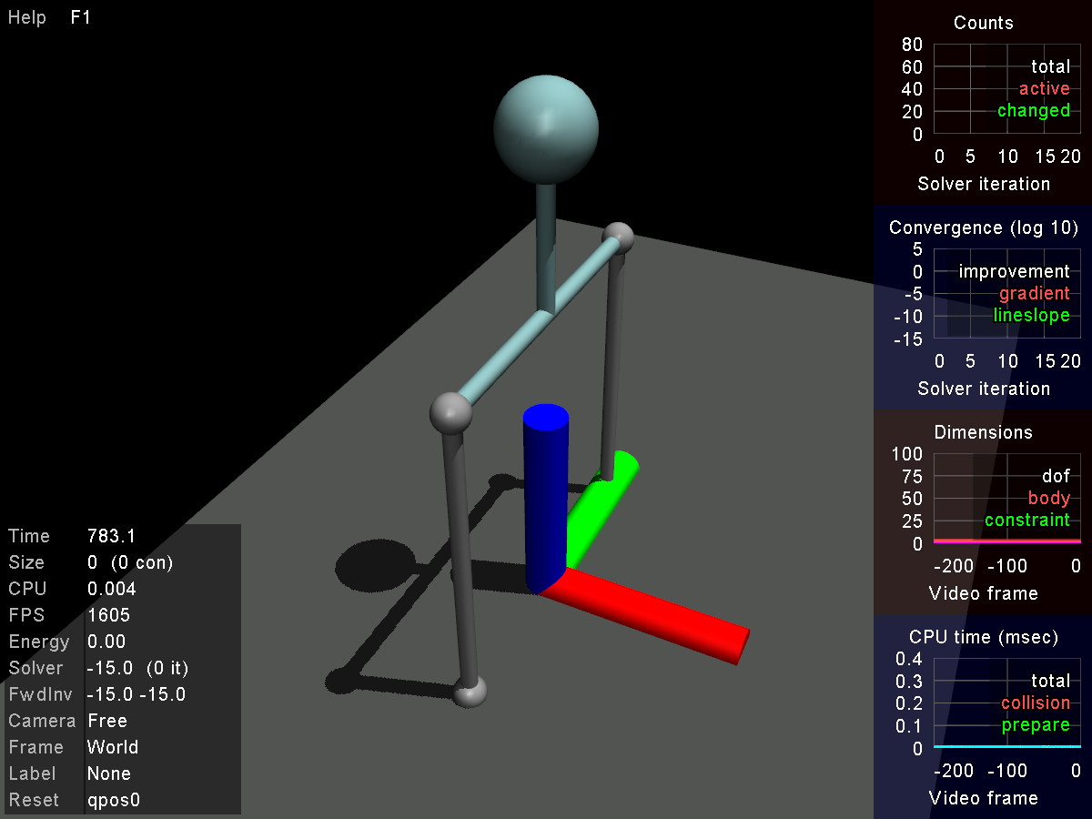
</actuator> If you simulate this file with basic program that comes with MuJoCo 2.0, i.e.:
$./basic $PATH_TO_ACROBOT.XML
you should see something like the following gif.
The initial configuration is selected such that our model conforms to Spong’s paper because he has provided us with the final LQR results. One important gotcha in using cylinders as bodies is how you define the properties of the cylindrical geoms which require radius and half-height. Also, regarding the orientations, make sure to have a look at this image which I uploaded to medium in my previous post. Finally, in this model I am not using sensors and in the code, we assume to have access to the correct measurements of states. I did not want to complicate this post more than it already is and I have already covered sensors in the medium post.
LQR controller of acrobot
I have prepared another SymPy code to calculate the linearized equations of motion of the robot around the up-right fixed point. We could have typed in these equations into our c++ file and substitute the values for mass, inertia, etc. from MuJoCo interfaces. This way we could have learned how to extract these quantities in MuJoCo, but I ended up avoiding this approach. The equations that SymPy spitted out are quite nasty to be written in a c++ code, moreover, we have estimated the equations as a Linear Time-Invariant (LTI) system which means matrices and (and consequently ) will not change with time or state.
It just made more sense to define these matrices in the beginning of the code with absolute numbers and ask Drake to calculate the Gain matrix for us.
Incorporating Drake into MuJoCo code
This step is actually very easy thanks to this repo.
You only need to follow the instructions here and if you found an issue with the output_port_value.h, look at this issue I opened for ways to handle it.
Here is the relevant portion of the code:
drake::systems::controllers::LinearQuadraticRegulatorResult getLQRControl()
{
  Eigen::Matrix<mjtNum , 4, 4> A_ = Eigen::Matrix<mjtNum , 4, 4>::Zero();
  Eigen::Matrix<mjtNum , 4, 1> B_ = Eigen::Matrix<mjtNum , 4, 1>::Zero();
  Eigen::Matrix<mjtNum , 4, 4> Q_ = Eigen::Matrix<mjtNum , 4, 4>::Identity();
  Eigen::Matrix<mjtNum , 1, 1> R_ = Eigen::Matrix<mjtNum , 1, 1>::Identity();
  Eigen::Matrix<mjtNum , 4, 1> N = Eigen::Matrix<mjtNum , 4, 1>::Zero();

// A
  A_.topRightCorner(2,2) = Eigen::Matrix<mjtNum , 2, 2>::Identity();

// Based on Spong
  A_(2,0) = 12.49;
  A_(2,1) = -12.54;
  A_(3,0) = -14.49;
  A_(3,1) = 29.36;

// B
  B_(2,0) = -2.98;
  B_(3,0) = 5.98;

// Q
//  Q_.topLefCorner(2,2) *= 10.0;  // optional
  return drake::systems::controllers::LinearQuadraticRegulator(A_, B_, Q_, R_, N);
}
Similar to what we did in the previous post, we can install a controller in MuJoCo by assigning a function to the mjcb_control function pointer simply by one-liner mjcb_control = mycontroller;.
Here is the barebone definition of mycontroller:
void mycontroller(const mjModel* m, mjData* d)
{
  mjtNum state[2*m->nq];
  mju_copy(state, d->qpos, 2*m->nq);
  state[0] -= M_PI_2; // stand-up position
  mjtNum ctrl = mju_dot(lqr_result.K.data(), state, 2*m->nq);

  d->ctrl[0] = -ctrl;

}
There are more prints in the repo version just to have a more informative controller. Also, because the initial position of the robot conforms to Spong’s formulation, I had to start the simulation close to the upright configuration. Feel free to play with the initial values to see how far your controller can stabilize the robot.
d->qpos[0] = M_PI_2 + 0.05;
d->qpos[1] = 0.0;
d->qvel[0] = 0.0;
d->qvel[1] = 0.0;
That’s all I have for now. Let me know below if you have feedbacks/comments and feel free to open up an issue if you had trouble compiling the code. See you next time with the swing-up control.